Swot L3_LR_SSH#
This chapter will present the functionalities specific to the Level 3 SWOT Low Rate products.
from fcollections.implementations import NetcdfFilesDatabaseSwotLRL3

import matplotlib.pyplot as plt
import matplotlib.patches as patches
import cartopy.crs as ccrs
Data samples#
We will illustrate the functionalities using a data sample from AVISO. You can use the altimetry-downloader-aviso tool to run the following script.
import logging
from pathlib import Path

from altimetry_downloader_aviso import get

logging.basicConfig()
logging.getLogger("altimetry_downloader_aviso").setLevel("INFO")

DATA_DIR = Path(__file__).resolve().parent.parent / "data"
DATA_DIR.mkdir(exist_ok=True)

if __name__ == "__main__":

    get(
        "SWOT_L3_LR_SSH_Basic",
        output_dir=DATA_DIR,
        version="2.0.1",
        cycle_number=[1, 2, 3],
        pass_number=[10, 11],
    )
Query overview#
Detailed information on the filters and reading arguments can be found in the
query API description
fcollections.implementations.NetcdfFilesDatabaseSwotLRL3.query()
The following examples can be used to build complex queries
A unique half orbit
fc.query(cycle_number=1, pass_number=1)
One half orbit repeating over all cycles
fc.query(pass_number=1)
A list of half orbits, over multiple cycles
fc.query(cycle_number=slice(1, 4), pass_number=[1, 3])
A time stamp
fc.query(time='2024-01-01')
A period
fc.query(time=('2024-01-01', '2024-03-31'))
A subset of variables
fc.query(selected_variables=['time', 'longitude', 'latitude'])
Note
Available variables can explored using
fcollections.implementations.NetcdfFilesDatabaseSwotLRL3.variables_info()
Zoom over an area selection
fc.query(bbox=(-10, 5, 35, 40))
Nadir and KaRIn data (Basic, Expert only)
fc.query(nadir=True)
Nadir data only (Basic, Expert only)
fc.query(swath=False, nadir=True)
Stacking over cycles (Basic, Expert, Technical only)
fc.query(stack='CYCLES')
Stacking over both cycles and passes (Basic, Expert, Technical only)
fc.query(stack='CYCLES_PASSES')
Fix a version
fc.query(version='2.0.1')
Choose one dataset
fc.query(subset='Expert')
Stack for temporal analysis#
The most prominent functionality is the ability to stack the half orbits when
the grid is fixed (Basic, Expert and Technical subsets). This allows
to work along the cycle_number dimension and compute temporal analysis
(mean, standard deviation, …).
There are currently three modes for stacking the half orbits
NOSTACK: do not stack the half orbitsCYCLES: concatenate the half orbits of one cycle along thenum_linesdimension, and stack the cycles along a newcycle_numberdimensionCYCLES_PASSES: stack the half orbits along thecycle_numberandpass_numberdimensions. Useful for regional analysis where the half orbits are cropped and we need an additional dimension to reflect the spatial jump
fc = NetcdfFilesDatabaseSwotLRL3("data")
ds = fc.query(stack='CYCLES', version='2.0.1', cycle_number=[1, 2, 3], pass_number=10, subset='Basic')
ds.ssha_filtered.data
|
||||||||||||||||
ds = fc.query(stack='CYCLES_PASSES', version='2.0.1', cycle_number=[1, 2, 3], pass_number=[10, 11], subset='Basic')
ds.ssha_filtered.data
|
||||||||||||||||
Note
Incomplete cycles are completed with invalids
Area selection#
It is possible to select data crossing a specific region by providing bbox parameter to query or list_files method.
The bounding box is represented by a tuple of 4 float numbers, such as : (longitude_min, latitude_min, longitude_max, latitude_max). Its longitude must follow one of the known conventions: [0, 360[ or [-180, 180[.
If bbox’s longitude crosses -180/180, data around the crossing and matching the bbox will be selected. (e.g. for an interval [170, -170] -> both [170, 180[ and [-180, -170] intervals will be used to list/subset data).
To list files corresponding to half orbits crossing the bounding box:
bbox = -126, 32, -120, 40
fc.list_files(
    version='2.0.1',
    subset='Basic',
    bbox=bbox)
| cycle_number | pass_number | time | level | subset | version | filename | |
|---|---|---|---|---|---|---|---|
| 0 | 2 | 11 | [2023-08-11T10:53:21.000000, 2023-08-11T11:44:... | ProductLevel.L3 | ProductSubset.Basic | 2.0.1 | /home/runner/work/fcollections/fcollections/do... |
| 1 | 3 | 11 | [2023-09-01T07:38:26.000000, 2023-09-01T08:29:... | ProductLevel.L3 | ProductSubset.Basic | 2.0.1 | /home/runner/work/fcollections/fcollections/do... |
To query a subset of Swot LR L3 data crossing the bounding box:
Note
Lines of the swath crossing the bounding box will be entirely selected.
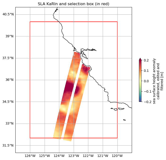
bbox = -126, 32, -120, 40
ds_area = fc.query(version='2.0.1', subset="Basic", cycle_number=2, pass_number=11, bbox=bbox)

# Figure
localbox_cartopy = bbox[0] - 1, bbox[2] + 1, bbox[1] - 1, bbox[3] + 1
fig, ax = plt.subplots(figsize=(8, 8), subplot_kw=dict(projection=ccrs.PlateCarree()))
ax.set_extent(localbox_cartopy)

plot_kwargs = dict(
    x="longitude",
    y="latitude",
    cmap="Spectral_r",
    vmin=-0.2,
    vmax=0.2,
    cbar_kwargs={"shrink": 0.3},)

# SWOT KaRIn SLA plots
ds_area.ssha_filtered.plot.pcolormesh(ax=ax, **plot_kwargs)
ax.set_title("SLA KaRIn and selection box (in red)")
ax.coastlines()
ax.gridlines(draw_labels=['left', 'bottom'])


# Add the patch to the Axes
rect = patches.Rectangle((bbox[0], bbox[1]), bbox[2] - bbox[0], bbox[3] - bbox[1], linewidth=1.5, edgecolor='r', facecolor='none')
ax.add_patch(rect)
<matplotlib.patches.Rectangle at 0x7f04914ac4a0>
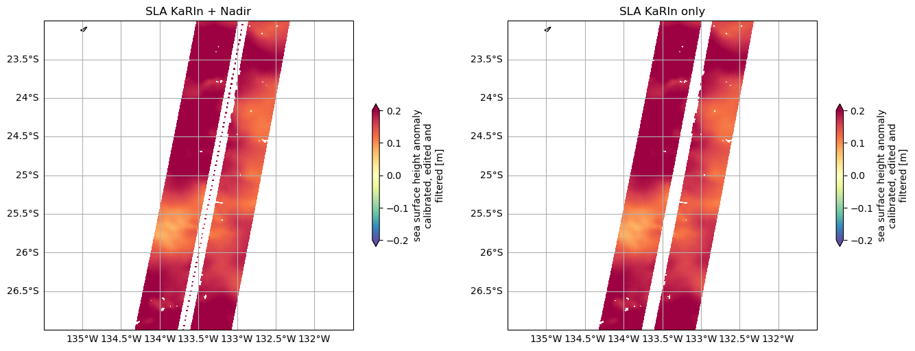
Handling nadir clipped data in Level-3 Basic and Expert subsets#
The L3_LR_SSH Basic and Expert subsets have the Nadir instrument data clipped in
the Sea Level Anomaly fields. The indexes where the nadir data has been
introduced are stored along num_nadir dimension. The SWOT implementation
offers various choices for handling this clipped data:
nadir=Falseandswath=True: remove the nadir data clipped. This is the default behaviornadir=Trueandswath=True: do nothing and keep both the KaRIn and Nadir instruments datanadir=Trueandswath=False: extract the Nadir instrument data only. This will give a dataset indexed along thenum_nadirdimension. Because it returns the nadir data only, we lose the possibility of stacking multiple half orbits
ds_full = fc.query(version='2.0.1', subset="Basic", cycle_number=2, pass_number=11, nadir=True)
ds_swath = fc.query(version='2.0.1', subset="Basic", cycle_number=2, pass_number=11, nadir=False)

# set figures
localbox = 224.5, 228.5, -27, -23
fig, (ax1, ax2) = plt.subplots(1, 2, figsize=(16, 9), subplot_kw=dict(projection=ccrs.PlateCarree()))
ax1.set_extent(localbox)
ax2.set_extent(localbox)

plot_kwargs = dict(
    x="longitude",
    y="latitude",
    cmap="Spectral_r",
    vmin=-0.2,
    vmax=0.2,
    cbar_kwargs={"shrink": 0.3},)

# SWOT KaRIn SLA plots
ds_full.ssha_filtered.plot.pcolormesh(ax=ax1, **plot_kwargs)
ds_swath.ssha_filtered.plot.pcolormesh(ax=ax2, **plot_kwargs)

ax1.set_title("SLA KaRIn + Nadir")
ax1.coastlines()
ax1.gridlines(draw_labels=['left', 'bottom'])
ax2.set_title("SLA KaRIn only")
ax2.coastlines()
ax2.gridlines(draw_labels=['left', 'bottom'])
<cartopy.mpl.gridliner.Gridliner at 0x7f048700f320>
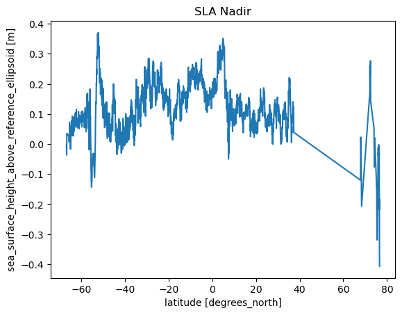
ds_nadir = fc.query(version='2.0.1', subset="Basic", cycle_number=2, pass_number=11, nadir=True, swath=False)

plt.plot(ds_nadir.latitude.values, ds_nadir.ssha_filtered.values)
plt.ylabel(f'{ds_nadir.ssha_filtered.attrs["standard_name"]} [{ds_nadir.ssha_filtered.attrs["units"]}]')
plt.xlabel(f'{ds_nadir.latitude.attrs["standard_name"]} [{ds_nadir.latitude.attrs["units"]}]')
plt.title("SLA Nadir")
Text(0.5, 1.0, 'SLA Nadir')